Copy page

• Copy page
• View source

---

• Open in ChatGPT
• Open in Claude
• Open in Perplexity

Styled Visualizations

This example showcases different plot styles and annotations. It demonstrates how sphinx-gallery captures complex matplotlib figures.

See also

• Basic Plot for a simpler example

• Subplot Layouts for subplot layouts

import matplotlib.pyplot as plt
import numpy as np

# sphinx_gallery_thumbnail_number = 2

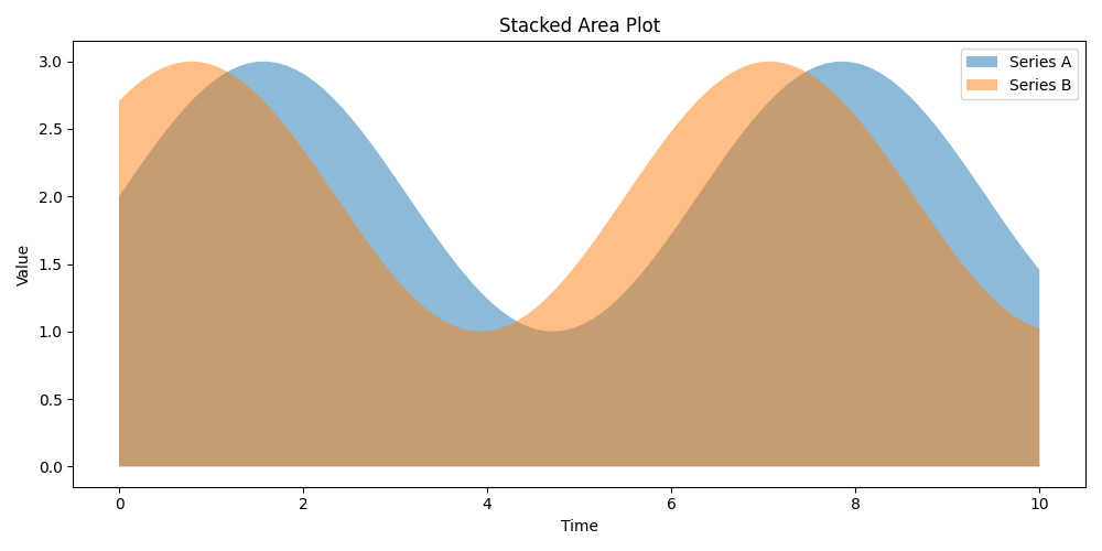
Area Plot with Gradient

A filled area plot showing data distribution over time.

x = np.linspace(0, 10, 100)
y1 = np.sin(x) + 2
y2 = np.sin(x + np.pi / 4) + 2

plt.figure(figsize=(10, 5))
plt.fill_between(x, 0, y1, alpha=0.5, label="Series A")
plt.fill_between(x, 0, y2, alpha=0.5, label="Series B")
plt.xlabel("Time")
plt.ylabel("Value")
plt.title("Stacked Area Plot")
plt.legend()
plt.tight_layout()
plt.show()

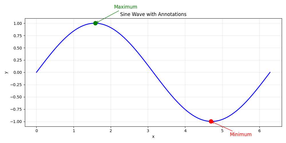
Annotated Plot

This figure includes text annotations and markers pointing to specific features. The sphinx_gallery_thumbnail_number = 2 directive at the top makes this the gallery thumbnail.

x = np.linspace(0, 2 * np.pi, 100)
y = np.sin(x)

fig, ax = plt.subplots(figsize=(10, 5))
ax.plot(x, y, "b-", linewidth=2)

# Mark maximum and minimum
max_idx = np.argmax(y)
min_idx = np.argmin(y)

ax.annotate(
    "Maximum",
    xy=(x[max_idx], y[max_idx]),
    xytext=(x[max_idx] + 0.5, y[max_idx] + 0.3),
    fontsize=12,
    arrowprops=dict(arrowstyle="->", color="green"),
    color="green",
)

ax.annotate(
    "Minimum",
    xy=(x[min_idx], y[min_idx]),
    xytext=(x[min_idx] + 0.5, y[min_idx] - 0.3),
    fontsize=12,
    arrowprops=dict(arrowstyle="->", color="red"),
    color="red",
)

ax.scatter([x[max_idx], x[min_idx]], [y[max_idx], y[min_idx]],
           c=["green", "red"], s=100, zorder=5)

ax.set_xlabel("x")
ax.set_ylabel("y")
ax.set_title("Sine Wave with Annotations")
ax.grid(True, alpha=0.3)
plt.tight_layout()
plt.show()

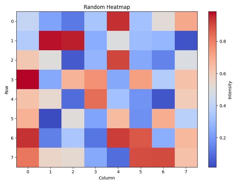
Heatmap

A 2D heatmap visualization with a colorbar.

data = np.random.rand(8, 8)

plt.figure(figsize=(8, 6))
plt.imshow(data, cmap="coolwarm", aspect="auto")
plt.colorbar(label="Intensity")
plt.xlabel("Column")
plt.ylabel("Row")
plt.title("Random Heatmap")
plt.tight_layout()
plt.show()